Complex (Cognitive) Systems - Autonomous University of the State of Morelos

work in progress...

This marvelous course by Prof. Markus Müller revealed like a hidden treasure in the most unexpected of places: a social-sciences and humanities-oriented postgrad program, in random underfunded university (the cognitive science masters degree from the Autonomous State University of Morelos, Mexico). The aim of self-publishing notes and assignments, and assembling them into a coherent whole, goes beyond giving everyone brave enough¹ a shot to enjoy it. It also sits as a personal reminder of my interest at the intersection of mathematical modeling, biophysics and the mind.

the brain meets the operational definition of what a complex² system is:

• hierarchical organisation, scale-free structure, many-to-many relations among components, interconnectedness (recurrence)
• non-linear behaviour, emergent properties (hard to determine from the observation of components alone, which number in the millions)
• chaotic to initial conditions (slight differences lead to widely different states)
• non-stationary measurements (dynamical system whose model constants/parameters actually vary; system doesn't stay in an attractor)
• phase transitions, equilibrium depends on critical states
• noisy measurements, plus some rather stochastic processes (spiking), whose measurable fluctuations may be difficult to distinguish from chaotic determinism

• dynamical systems basics

we'll distinguish between two kinds of systems:

• stochastic
• dynamical (deterministic). e.g. the harmonic oscillator:

• harmonic oscillator

consider the mechanics of a mass attached to a spring (no other forces involved, e.g. friction, gravity). let's say this is a very simple brain model (or of one of its components thereof) whose activity behaves like an oscillating variable:

from Newton's second law and Hooke's law:

therefore³

in order to solve the second-order linear ordinary homogeneous differential equation, we partition it into a system of two first-order equations. let , therefore:

notice that with the last substitutions both equations are the same, except in terms of different variables. both sin(ω₀t) and cos(ω₀t) satisfy it, because:

and

more generally, solutions will conform to the linear superposition principle:

any possible function of position on time will look sinusoidal, of varying frequency (depending on ), amplitude and phase (a and b together). we rewrite it as:

this has the property that , and .

let be the initial phase. then

so:

graphically:

• initial conditions

finally, let's say the spring is totally relaxed at t=0, so . this implies that :

• complex polar notation

prove that is the unit circle.

following Euler's formula, . therefore ⁴

solutions of the form include the aforementioned trigonometric solutions when λ, A ∈ ℂ. so the #original differential equation can be rewritten as:

the general solution becomes:

if we restrict x(t) to the type ℝ→ℝ (position is real), it follows that x(t) equals its complex conjugate.

moreover, . this implies that and . so:

compare this expression against the one using trigonometric functions.

• energy loss

(also see #dissipative systems and attractors)

now we will damp the oscillator by adding a term for friction, whose force is proportional to velocity (but in opposite direction):

assume a family of solutions of the form . therefore:

plug that back into the general solution:

asymptotically, the system will inevitably evolve to the most entropic dynamic state. let's show this on a case-by-case basis, taking note on the different (non)monotonic dynamics:

• underdamped: ω₀ > β

let :

by restricting x(t) to ℝ→ℝ, and from our previous knowledge of the simple harmonic oscillator solution:

• ω₀ = β

we leverage the fact that amplitude isn't constant anymore:

and the damped harmonic oscillator equation becomes:

i.e., amplitude is a linear function. so the solution must be of the form:

graphically, the spring oscillates only once:

• overdamped: ω₀ < β

because , is overshadowed by . the plot never gets to complete an oscillation:

• energy input

the damped model will get augmented with the influence of external stimuli, driving our cognitive-unit model to activity. this is known as a driven harmonic oscillator. let's go with an engine rotating at frequency and amplitude F, which in turn pushes and pulls the rest of the system:

the equation isn't homogeneous anymore. the solution is the sum of the general and particular solutions: the homogeneous one is of the type and eventually dissipates. the particular one oscillates forever:

• resonance

starting from an exploration of the steady state ("final conditions"), we will show that amplitude is a function of the engine's frequency, and that there are privileged frequencies for which steady-state amplitude forms maxima or singularities: resonance frequencies.

so we rewrite the full differential equation:

(...magic happens here...)

• phase space

phase space contains all information of a dynamical system, with a different axis for each variable of interest. each point in it represents a state of the whole system, and a trajectory in this virtual space corresponds to the evolution of the system.

signal: disregarding noise, taking a series of measurements is equivalent to observing variation in a single dimension of phase space. graphically, this is a projection of the system upon some vector in phase space.

• Fourier analysis

• linear independence of Fourier terms

let with be functions on the interval . prove that , given the proper definition of the dot product. is Dirac's delta distribution.

let be the scalar product for functions of the vector basis defined by .

proof by modus ponens follows:

• restatement of conditional premise

given the above definitions; if , then is an orthogonal basis. that is:

• proof of the antecedent premise

indeed:

because:

from Euler's formula:

from the integration of the odd function over a zero-centered interval, :

let ; then .

note that .

• conclusion

is an orthogonal basis.

• Fourier transform

the Fourier series represents a periodic function as a discrete linear combination of sines and cosines . on the other hand, the Fourier transform is capable of representing a more general set of functions, not restricted to being periodic. how is that achieved?

(for convenience, we will start from the series in complex exponential notation)

if weren't periodic, the series would be representing it only at . nonetheless, we can make the interval arbitrarily large:

let , then . substituting in the last expression yields:

which is a Riemman sum for variable :

• properties

which symmetry properties does H(f) has if h(t) is:

1. odd real
2. odd imaginary
3. odd complex

and which symmetry properties does h(t) has if H(f ) is:

1. odd real
2. even complex
3. even imaginary

recall that:

• odd real h(t)

we get rid of the imaginary part of H(f):

from integration of an odd function (r(t)cos(2πft)) at a symmetric interval:

is odd. is odd and imaginary.

• odd imaginary h(t)

same reasoning:

is odd. is odd and real.

• odd h(t)

is odd. is odd and complex.

• odd real H(f)

is odd. is imaginary and odd.

• complex even H(f)

is even. is even and complex.

• imaginary even H(f)

is even. is even and imaginary.

• uncertainty principle

the more short-lived the wave in the time domain, the more widespread its power spectrum (a.k.a. frequency spectrum). vice versa.

• convolution theorem

is the convolution of functions x(t) y h(t). F[y(t)] denotes its Fourier transform:

let u=t-τ.

therefore:

time-domain convolution is equivalent to frequency-domain product!

• cross-correlation theorem

is the correlation (covariance, actually) of functions x(t) y h(t) as a function of a time lag between them. F[z(t)] denotes its Fourier transform:

let u=t+τ.

therefore:

cross-correlation is equivalent to frequency domain product (with conjugate X(f)).

• discrete Fourier transform

the computation of a DFT is done segment by segment. the signal is multiplied by some "window" function (e.g. a square pulse) which is zero outside the window. this is known as windowing.

the effect of using a finite window is that unexisting frequencies appear at the power spectrum (around the original frequencies). this phenomenon is known as leakage. the explanation is evident from the #convolution theorem: one can use similar reasoning to show that . therefore, multiplication by a window will induce a convolution in the frequency domain.

low frequencies (and therefore #non-stationary systems) are the most problematic to compute a DFT for, since the window may not be long enough to capture them. there's no single #test for stationarity. it can be tested for nonetheless, measuring the effect of varying window sizes on different parameters (centrality and spread statistics, Lyapunov exponent, etc.).

• Whittaker–Shannon (sinc) interpolation

what function should we convolve the signal's Fourier transform with in order to obtain the same result as windowing it with a rectangular function? we will analyze the closely-related case of a square pulse window:

calculate the first three terms of the Fourier series for function , with

in terms of the Fourier series:

from the integration of odd functions ( and ) at symmetrical interval ( ):

we will consider the interval , which includes a full period of for any n. therefore:

f(x) could be just a discrete sample of a continuous signal, but because convolution with sinc(x) produces a continuous function (a sum of sine waves), the operation will fill in all the missing time points.

• Nyquist-Shannon sampling theorem

continuous functions of bounded frequency bandwidth ("band-limited") contain a bounded amount of information. they can be perfectly represented using a function of countable (i.e. discrete) sets and an interpolation operation.

the Nyquist frequency is the maximum sampling frequency at which the digitization of a continuous signal still losses fidelity. that is, aliasing occurs:

sampling frequency should be greater than twice the maximum frequency in the power spectrum of the original signal.

undersampling results in the unconsidered high frequencies aliasing (adding up) over at the frequency domain. oversampling is harmless, beyond being a waste of disk space.

• testing for undersampling

what if the maximum frequency isn't known in advance? it is possible to test that the maximum frequency has been considered, because aliasing will make two power spectra of the same signal look dissimilar under two different sampling frequencies:

1. register using two sampling frequencies, one greater than the one to test for the Nyquist criterion.
2. compute both power spectra ( ).
3. if they are simply scaled versions of one another, aliasing didn't occur. i.e. the ratio between two features (e.g. maxima) should stay constant.

• other time-series topics

• stochastic correlations

suppose the signal is generated by an stochastic process. if low frequencies dominate the power spectrum, then the process is non-stationary (time-series mean value will be trending over long periods of time) and autocorrelation will be large.

corollary: even two independent sources of noise can display high statistical dependence.

averaging the time series would be no good. prediction should take autocovariance times into account, detrending methods are also available.

• stationarity

• strict/particular stationarity: system's parameters are truly constant. too hard a requirement, since we must know the system's differential equations in advance.

• weak/general stationarity: empirical transition probabilities in the F map stay constant. affected by low-band frequencies. alternatively, 1st moment and autocovariance stay constant and finite. this requires greater data availability, because short acquisition times may not be enough to establish statistical relevance.

• linear prediction

suppose there's a time series whose value we want to predict. in a linear prediction algorithm we define as a linear combination of the last m points:

it's clear that there are as many linear combinations of the last m points as there are permutations (with substitution) of coefficients . in order to find the optimal coefficients we try to minimize the mean square error predicting the previous m - 1 values:

• cross-validation

• in-sample accuracy: estimated from predictions made for the same data segment used during training/optimisation phase. it doesn't reflect the algorithm's true predictive power (overestimate), since tests aren't predictions but "post-dictions".
• out-sample accuracy: error estimated from true predictions, using the values of data never "seen" before by our predictive model.

• phase-space methods

• dissipative systems and attractors

dissipative system: on average, the volume of the manifold describing the state trajectory contracts under dynamics, after certain initial conditions. alternatively, it can be said that #energy loss creates an attractor for that system, reducing the set of possible states that it can take with time. nonetheless, the system still operates far from thermodynamic equilibrium.

in order to verify the presence of an attractor, the L1 metric of the determinant of the system's Jacobian (i.e., of the state transition function's (F) partial derivatives) must be smaller than 1, on average:

this means that the transformation's scaling factor produced by change on the different directions is a contracting one. visually, if phase space contains an attractor then the system is dissipative.

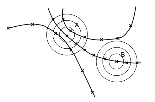
• visual inspection

• Poincaré section: allows to tell whether the trajectory behavior is classically deterministic, chaotic deterministic or random. it amounts to finding the intersection between trajectories and a secant plane.

• stroboscopic map: graphical representation of Poincaré's section technique for attractors. section is adjusted until the scatter plot is maximally decorrelated. also used for qualitative detection of strange/fractal attractors.

• "phase portrait": also known as delay representation. it is a bidimensional representation of any m-dimensional phase space. each point is given by a pair of subsequent states in phase space (see also #Takens-Whitney embedding theorem). it eases the visualisation of multidimensional systems and helps identify determinism, periodicity, linearity and chaos.

• Takens-Whitney embedding theorem

it is possible to reconstruct a phase space manifold that is isomorphic to the original one, even when all information we have is a time series, through the method known as delay reconstruction.

requirements:

• stationary data
• low-dimensional system
• negligible noise

the basic idea is that for each subset of m equidistant points in the signal, there's an associated unique point in m-dimensional phase space. each value in this subset of the time series becomes a component of the state vector:

note that the closer and are, the more correlated the reconstructed attractor; rendering it less useful:

the spacing parameter among points in the time series is called the time lag τ. to set an adequate value for τ, we want τ > L; with L being the autocovariance length. that is, we want the time between two measurements to be long enough so that they aren't correlated anymore.

finding the right number m of dimensions involves increasing the number of embedding components per point, until the manifold can't unfold anymore. we say there are false neighbors (and therefore that the embedding isn't high-dimensional enough) whenever an increase in m separates seemingly close points considerably in reconstructed phase space.

• non-linear prediction

unlike the #linear prediction algorithm for time series; a non-linear algorithm doesn't use the last m points combined. rather, it builds upon the intuition that the most relevant states for making a prediction some time Δn after the present are the ones that most resembled the current state. it then averages those similar states after Δn:

where denotes the cardinality of the current state vector's neighborhood (in phase space).

• as stationarity test

1. divide the series in intervals so short so as to have lineal segments.

2. predict and cross-validate using all possible segment pairs.

3. if some training segments display unusually different performance, then they don't generalise to the whole series. therefore we can conclude that the attractor changed as we swapped training segments; and the time series isn't stationary.

• as a noise smoother

suppose the measured time series is the sum of its true value and noise:

where is the random component. also suppose and are independent, and that temporal correlation is short.

we want to substitute with . starting from the #non-linear prediction algorithm:

1. in phase space, use trajectories which are close to the current one (both in the past and future portions), since the points inside that neighborhood belong to an n-dimensional sphere with center at the vector state under consideration.

2. apply the nonlinear prediction algorithm afterwards: average the vectors in the neighborhood. thus the stochastic component will be largely cancelled out.

• chaos theory

• Lyapunov coefficient

quantifies chaos levels in a dynamical system. it is the exponent in the exponential divergence measurement of phase space. the system has as many Lyapunov exponents as dimensions, positive ones are chaotic dimensions:

Lyapunov coefficient	kind of attractor
λ < 0	stable fixed point
λ = 0	stable limit cycle
λ > 0	chaos
λ → ∞	noise

• estimation from time series

it is advisable to perform a #phase portrait beforehand, so as to rule out that the system is nondeterministic.

caveats:

1. embedding: if the #embedding dimension is too low divergence will be underestimated because of false neighbors.
2. noise level: overestimated because of noise
3. #stochastic correlations: if autocorrelation is big, the attractor will look compressed along a diagonal, underestimating true divergence

• fractal dimension

strange attractors are the flagship of chaos: trajectories are still deterministic (no crossroads) yet non-cyclic (exact knowledge is required to tell accurately which trajectory the system is in). since some chaotic systems are also #dissipative, all of this implies that a subset of infinitely-dense phase space is being relentlessly filled by a line of infinite detail.

• box counting

box counting is one of many methods to assess scaling property of fractals.

let ε be the side of each box (n-dimensional squares), which are in turn used to segment the figure. then let N(ε) be the number of boxes. note that:

D being the box-counting fractal dimension.

Example:

N(ε)	ε
30	20
31	21
32	22
...	...
3n	2n

• correlation dimension

the correlation dimension can be used as an estimator of an attractor's dimension.(under certain circumstances), including fractal dimensions.

the idea now isn't to take the ratio of the number of boxes and their length ε in the limit to infinity. instead, we take the ratio of points (among all possible valid pairs) which fall within the neighborhood (defined by a radius of length ε) of some other point:

where C(N, ϵ) is the correlation sum:

𝛩 is Heaviside's step function

• estimation from time series

given the lack of a phase space, it is necessary to #reconstruct it first. the right choice of delay τ during reconstruction of embedded vectors provides a suitable delay to estimate correlation dimension.

the aforementioned estimator of C(m, ϵ) is biased to underestimate the dimension, because data that are close in a trajectory of phase space tend to retain some temporal correlation.

the corrected estimator of C(m, ϵ) excludes sufficiently-close vector pairs (in phase space); which usually correspond to subsequent vectors in the time series:

with . doesn't necessarily have to be the average correlation time.

the following plots from Kantz & Schreiber's book⁵ come from a map-like system. for a only 2.5% of all pairs is lost in the corrected correlation dimension estimator. this is statistically negligible.

possible error sources:

• the correlation is a well-defined construction (for finite data sets), whereas the correlation dimension is just an extrapolation that must be handled with care.
• it isn't enough to observe fractal scaling for a single choice of m. saturation should also occur for many values.
• if measurements are too noisy, a scaling regime may never be observed. the dimension estimate can be as big as m whenever ϵ is small enough, so that only noise is captured by it.
• noise affects scales 3 orders of magnitude as big as its own level. in order to observe a scaling region, noise should be at most 1/8 of the whole attractor.
• it is therefore advisable to use a #noise reduction algorithm in advance.
• certain stochastic systems may pass for low-dimension deterministic systems.
• low-resolution digitization will make the estimate look smaller
• self-similarity may never be observed, even for good-quality deterministic data, depending on the manifold's large-scale structure.

• minimum delay

a space-time separation plot shows the proportion of points inside the neighborhood as a function of Δt and ϵ. we hope to find some value of Δt after which increments in ϵ don't add extra points. such delay marks the ideal choice of Δt when computing the correlation sum.

this is more rigorous a technique than using the autocorrelation distance.

• as a noise meter

figures 19 and 20 introduced the value ε that marks the limit between noise and scaling regimes. we found a resolution limit in the data, when neighborhoods were so tiny that they only capture randomly distributed points in all directions.

in a nutshell, given that ε is a distance in phase space units, we can define the noise level as the ratio between ε and the attractor's "size".

• neuroscience applications

• how not to use it:

Lehnertz and Elger (1998)⁶ analysed localized intracranial EEG data from 16 epilepsy patients. they claimed that a loss of complexity in brain activity should result from the synchronization of pathological cells before and during seizures.

linear techniques can only predict seizures a few seconds in advance. here the intention is to use the correlation dimension estimate as a complexity detector, even though it cannot actually estimate the fractal dimension for these data.

a state called state 2 coincides with pre-ictal synchronization some 10 to 30 minutes in advance to the seizure. nothing is mentioned with regard to confounding sources of complexity reduction, though.

quasi-scaling regions were observed for state 2 (D₂^eff = 3.7) and the seizure state (D₂^eff = 5.3), but not the control state. in other words, complexity apparently increased, counter to theory, and there's no base level to compare it with.

plots don't really show a clear power law either that would justify the reliability of their estimates. nor was any statistical hypothesis test performed using surrogate data.

• a more credible one?

Martinerie et al (1998)⁷ attempted to predict seizures by looking at phase transitions between two subsections in reconstructed phase space, also built from intracranial EEG series. it is claimed that for most cases (17 out of 19) it is possible to foretell seizure onset 2 to 6 seconds in advance, and that all of them follow a similar trajectory in phase space.

the alternative hypothesis is actually explored with surrogate data, and authors made sure to smooth noise out previous to the embedding. the number of dimensions (16) may be too unwieldy, though.

• hypothesis testing

the maximal Lyapunov coefficient and the correlation dimension come handy in detecting non-linear dynamics, however they cannot establish such a fact by themselves. it is necessary to observe a clear scaling region.

a stricter analysis would test the hypothesis that observed data are due to a linear process. this implies that certain parameter's conditional distribution (given H₀) has to be empirically estimated, so that it can be contrasted with the real data.

• surrogate data

surrogate data is a akin to resampling methods (permutation, Monte Carlo, bootstrapping) for time series. surrogate data share many similarities with true data for some respects, while consistent with H₀ for others. when testing for non-linearity, Fourier phases are generated randomly while the power spectrum is retained, since the imaginary part is where non-linearity could emerge from.

the general procedure for generating surrogate data is as follows:

1. decompose the signal in amplitudes and phases using the (fast, discrete) Fourier transform:

2. substitute the alleged non-linear properties with random numbers drawn from the uniform distribution ranging from 0 to 2π radians (trying to make , so that the imaginary part being odd will result in a substitute series belonging to ℝ. see the #Fourier transform properties section):

3. wrap the surrogate series back with the inverse Fourier transform:

4. test the series out (dimension estimation, Lyapunov coefficient, autocorrelation, non-linear prediction error, etc.).

5. rinse and repeat till the parameter's distribution given H₀ is dense enough to yield good type-I error estimates.

• statistical significance

as in standard hypothesis testing, for a significance level of α (type I error: probability that H₀ is erroneously rejected) we would like at most α% of the area under the surrogate data curve to overlap the original measurements, or be equal or more extreme than our point measurement. such a rank-based test is a non-parametric way of deriving a p-value.

for instance, in order to reject H₀ with 95% of success, it would be enough to perform tests (for a one-side test. for the two-tail case).

• as a determinism detector

does passing the test also mean that the system is deterministic (since we tested for non-linear determinism)?

partially yes, with some probability. recall that all statistical inference is based on limited evidence and inductive reasoning:

	accept H0	reject H0
H0 is true	1-α (confidence)	α (type I error)
H0 is false	β (type II error)	1-β (power)

more caveats:

• we have assumed that the available power spectrum captures at least one whole period in the time domain (i.e. no systemic sampling bias due to long-term process). otherwise, random events in a non-stationary process could be misinterpreted as deviations from H₀.
• the process may not follow the conjectured probability distribution (this problem is mitigated by non-parametric tests).
• multiple comparisons problem: performing many independent tests overblows type I error. for those cases, significance levels should be made more stringent according to some correction method (Bonferroni e.g.)

• as a phase transition detector

the same non-linearity tests have been used to distinguish states of a system.

compute the same statistic for different time segments and compare with one another. the reasoning follows what we did in the #stationarity test.